The topic describes the most common reasons for "#N/A error" to appear are as a result of either the INDEXor MATCH functions.
Note: If you want either the INDEX or MATCH function to return a meaningful value instead of #N/A, use the IFERROR function and then nest the INDEX and MATCH functions within that function. Replacing #N/A with your own value only identifies the error, but does not resolve it. So, it's very important, before using IFERROR, ensure that the formula is working correctly as you intend.
Problem: There is no data to match
When the MATCH function does not find the lookup value in the lookup array, it returns the #N/A error.
If you believe that the data is present in the spreadsheet, but MATCH is unable to locate it, it may be because:
-
The cell has unexpected characters or hidden spaces.
-
The cell may not be formatted as a correct data type. For example, the cell has numerical values, but it may be formatted as Text.
SOLUTION: To remove unexpected characters or hidden spaces, use the CLEAN or TRIM function, respectively. Also, verify if the cells are formatted as correct data types.
You have used an array formula without pressing Ctrl+Shift+Enter
When you use an array in INDEX, MATCH, or a combination of those two functions, it is necessary to press Ctrl+Shift+Enter on the keyboard. Excel will automatically enclose the formula within curly braces {}. If you try to enter the brackets yourself, Excel will display the formula as text.
Note: If you have a current version of Microsoft 365, then you can simply enter the formula in the output cell, then press ENTER to confirm the formula as a dynamic array formula. Otherwise, the formula must be entered as a legacy array formula by first selecting the output range, entering the formula in the output cell, and then pressing CTRL+SHIFT+ENTER to confirm it. Excel inserts curly brackets at the beginning and end of the formula for you. For more information on array formulas, see Guidelines and examples of array formulas.
Problem: There is an inconsistency in the match type and the sorting order of the data
When you use MATCH, there should be a consistency between the value in the match_type argument and the sorting order of the values in the lookup array. If the syntax deviates from the following rules, you will see the #N/A error.
-
If match_type is 1 or not specified, the values in lookup_array should be in an ascending order. For example, -2, -1, 0 , 1 , 2…, A, B, C…, FALSE, TRUE, to name a few.
-
If match_type is -1, the values in lookup_array should be in a descending order.
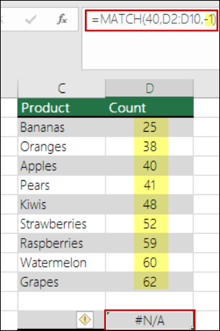
In the following example, the MATCH function is
=MATCH(40,B2:B10,-1)

The match_type argument in the syntax is set to -1, which means that the order of values in B2:B10 should be in descending order for the formula to work. But the values are in ascending order, and that causes the #N/A error.
SOLUTION: Either change the match_type argument to 1, or sort the table in descending format. Then try it again.
Need more help?
You can always ask an expert in the Excel Tech Community or get support in Communities.
See Also
How to use the INDEX and MATCH worksheet functions with multiple criteria in Excel


